• Welcome
• LCD Displays
  • Backlight
  • Liquid Crystals
  • IPS Technology
  • Brightness and Contrast
  • LCD References and Links
  • Bits and Color
  • Monitor Gamma
  • Gamma References and Links
• Monitor Color Management
  • Calibration & profiling
  • Colorimetric characterization
  • Examples of characterization
  • Examples (Part 2)
• GammaCalc
• Scanning
  • Scanner Types
  • Scanner Hardware
  • Density, D, Dmax
  • Scanner Calibration
  • Scanner Profiling
  • Scanning Workflows
• Color and Colorimetry
  • CIE XYZ and chromaticity
  • Light sources & illuminants
  • Chromatic adaptation
  • Transformation of RGB primaries
  • CIELAB color pace
  • Color differences
  • Glossary of terms
• Software Tips
  • BabelColor CT&A and PatchTool
  • Imatest and Gamutvision
  • Argyll CMS
  • ProfileMaker5
  • ColorThink Pro - soon
  • HCFR Colorimeter
• Search
•  

Gamma:

Several authoritative and very insightful papers and web sites were written on the subject of gamma (ref). However, definitions and interpretations still remain a subject of continuing discussion. Instead of going into the merits and controversials of gamma encoding/decoding/compensation, I will focus on its principles, application, and measurement.

To at least introduce the topic, let's start with simple empirical observations that will lead us to more intuitive meaning of the gamma. Our everyday experience points to the fact that human senses, such as hearing, sight, smell, and heat respond and adapt to extremely wide ranges of stimuli. To cope with such a large dynamic range, our hearing system, eyes, nose, and sensory neurons in skin evaluate the corresponding stimuli on nonlinear (approximately logarithmic) scale. Simply, when we double the light intensity, we don't see the light as twice as bright! The magnitude of a physical stimulus and its perceived intensity or strength follows the Stevens' power law (Fig. 14). Stevens' formulation is widely considered to supersede the famous Weber-Fechner law on the basis that it describes a wider range of sensations. Mathematically, the Stevens' law is formulated as follows:

R = k . (S-S0)p

Logarithm of both sides of this equation leads to a linear relationship between log(S-S0) and log R, with slope of the line determined by p. Figure 14 illustrates the qualitative relationship between stimulus of the human sensor system (S) and the response that we feel (R). Dashed line (p =1) would correspond to the linear dependence.

Figure 14: Stimulus intensity vs. objective response

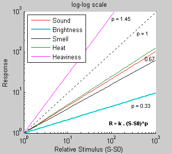For example, the way we feel heaviness of an object is characterized by a high value of p, reflected in a steep curve. In other words, once a stimulus is strong enough to sense "heaviness" of the object, the perception of "heaviness" rapidly becomes stronger as the stimulus becomes stronger. The other sensory responses shown have lower p value, which means that they can cover much wider ranges of stimulus intensity (dynamic range). Perception of light brightness has particularly low power exponent, which indicates that our vision system adapts to a wide dynamic ranges of the light. We will see the coefficient 0.33 (1/3) later in the context of perceptually uniform lightness scale as defined in the CIELAB color space. The sensitivity of the human eye is influenced by the average light level to which the eye is exposed.

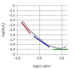
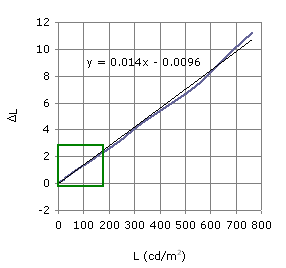
Representative result of noticeable luminance-difference measurements performed in the range of typical LCD luminances is shown in Fig. 15. The quantity log(ΔL/L) is plotted against the log(L) where L is luminance in cd/m2 (correlates with relative brightness). Some theoretical approaches predict a three-segmented curve, with slopes of -1 (the linear range), -0.5 (the square root range), and 0 (the Weber range). The same data on the linear scale is shown in Fig. 16. For luminance levels of interest (0.1 - 200 cd/m2), the ratio of ΔL/L has approximately constant value of 0.01 (so called Weber-Fechner fraction). Fit to a line with the slope of ~0.01 is remarkably good. In this region, the just noticeable difference in luminance (JND ~ ΔL) then follows the linear equation: ΔL = 0.01 * L. This relationship just confirms the empirical observation that we are more sensitive to luminance changes in the darker levels (at L = 100, JND = 1 while at L = 10, JND = 0.1). This observation will be mentioned later when gamma encoding is discussed. It is important to note that sensitivity of human vision varies with the light level and that in order for us to discriminate between two close luminance levels, one has to be fully adapted to the surround luminance. To be able to distinguish shades of gray in darker areas, our eyes have to be completely adapted to a lower intensity environment (globally as well as locally). For additional information on this topic, refer to the paper "Gamma and its disguises" of Charles Poynton and see the section "Why gamma" at Norman Koren's web pages.

Figure 15: Log-Log scale

Figure 16: Linear scale

In contrast to the human senses, linear data representation is widely used for computer generated imagery, mostly because models of illumination, white-point conversion, RGB color conversions, and color matching are defined linearly. Furthermore, the image sensors (CCD or CMOS) are linear devices that respond proportionally to the number of photons that interact with their electrode structure.

Quantization:

At the outset of the gamma discussion, the topic of quantization will be briefly discussed. In order to render captured scenes faithfully, digital devices have to have the ability to adequately sample (quantize) dynamic ranges of typical everyday scenes. Digital imaging systems with usually a limited number of bits (typically 8) must be designed so that there is enough precision in the low levels (shadows) to avoid visible contouring (our eyes are quite sensitive to transitions in shadow areas - Fig. 16). This can be achieved by applying a logarithmic or gamma-law "correction" to the linear data (logarithmic quantization has often been recommended but rarely implemented). Such transformations usually proceeds in two steps. First, the image is converted by analog-to-digital converter to, e.g., 12 bits in uniform steps (4,096 steps). Second, the output signal is then reduced to 8 bits by a nonlinear transformation that leads to compression of high level bins. When working with a typical LCD display that has about a 300:1 contrast ratio, our eyes can distinguish about half of the luminance levels. For 8-bit grayscale gradient, there would be theoretically 8.2 f-stops (exposure zones, log2300 = 8.2). For all 256 levels, there would be about 256/8.2 = ~ 31 distinguishable levels per a zone. As a result of interference from higher luminance levels (flare, bright environment), our capacity to distinguish levels in darker areas is compromised. Coming back to the Weber-Fechner law, the theoretical number of distinguishable levels per exposure zone is equal to log(2)/log(1.01) = 70. Number two relates to the exposure zone definition (half or double of the light intensity) and 1.01 is the 1% JND difference coming from the Weber-Fechner law. Again, this number of levels assumes complete adaptation to relatively narrow range of luminances around the evaluated neighboring levels.

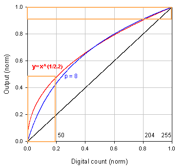
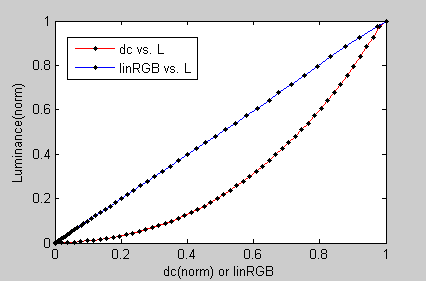
The idea behind nonlinear quantization is depicted in Figure 17. The x-axis is normalized digital input such as a photon count passed through the analog-to-digital converter (ADC). Numbers just above are the input values for 8-bit encoding (typical image editing range of 0-255). Black line is the linear response of an arbitrary digital device (camera, scanner sensor). Clearly, the output (on the y-axis) is directly proportional to the input. As an example of logarithmic correction, the blue curve in Fig. 17 describes transformation from the linear (black) to a logarithmic domain. In order to avoid log troubles at 0 , transformation (I) was used instead of direct log. Dc is the digital count input and p is a parameter ∈ (0, ∞).

The red curve is a "classical" simple gamma-corrected linear mapping. One can see that gamma mapping is steeper in shadows while highlights have nearly identical mapping. If we were quantizing in linear steps, we would be "wasting" bits in bright regions (remember, we can't distinguish much of the brightness level difference in lights anyway) and not having enough in areas where it matters most, i.e. darks. Here is why. For the linear scale, pixels above value of 204 (in 8-bit encoding) would require (1.0-0.8) x 100 = 20% of the available bits (same as pixels below 50). For the nonlinear scale, same regions will claim ~10% ((1.0-0.9) x 100) and 50% of available bits, respectively (orange rectangles). Read the following box and references for more examples and explanations.

Figure 17: Effect of quantization in a capture device

Clear benefit of these transformations is that the number of bits required to eliminate contouring of camera images in a computer display can be reduced from the "safe" 10-12 bits for linear data to 8 bits for logarithmic or gamma-corrected data (see the note above). This has beneficial impact on signal storage and transmission. Also, such nonlinear ("gamma") correction mathematically transforms the physical light intensity into a perceptually-uniform domain. Furthermore, it just happens that operating principle of CRT displays requires a gamma correction close to 1/γ to maintain perceptual and pleasing tone uniformity. So, the first gamma compressed the signal in a capture device, while the second gamma effectively decompressed the corresponding image (Fig. 18), keeping it perceptually similar to the original scene. It is the second gamma that we are mostly concerned with when processing and manipulating digital images. Figure 18 depicts the typical display gamma relationship between digital RGB values (normalized at x-axis) and the luminance output (red curve). Once the input digital counts are linearized, linear relationship between input and luminance becomes apparent (blue line). In general, linearization can be achieved by any of the mathematical models described in the next section or by canceling out the gamma and 1/gamma curves shown in Figures 17, 18 (red lines). An example of such cancellation is the so called overall system gamma (viewing gamma) that can be also computed by multiplying the camera gamma by the display gamma (γ_overall = γ_camera * 1/γ_display ~ 1). In reality, this overall gamma is typically in range of 0.96-1.30. The simple camera gamma is equal to 1/2.2 = 0.4545. Display gamma is gamma that we are concerned with when setting the calibration target. For Windows system its value is typically 2.2. It is important to note that gamma only affects middle tones and has negligible effect on dark or white areas.

Figure 18: OETF curve and its linearized form

Unfortunately, the term gamma is used rather ambiguously and it is always necessary to verify how the particular gamma is defined. For display devices which we are most interested in, the correct term for (or meaning of) gamma is the tone reproduction curve (TRC). It is also known as the optoelectronic transfer function (OETF) and in general, it describes the relationship between the signal sent to a display (from the video frame buffer ) and the radiant output produced by each RGB channel. This relationship is usually nonlinear (as discussed above) and must be somehow modeled or predicted in order to characterize any particular display device. Technically, for LCD displays, this relationship is not an easy function, but rather results of curve-fitting to representative input points that are stored in profile or calibration lookup table (LUT). This LUT typically involves 16-bit data mapping. Strictly speaking, it follows that there is no "gamma" for LCD displays as there is no "power function" physics behind the LCD luminance output. While electron guns in CRTs have smooth power-function characteristics along the whole tonal range of each RGB component, the native response of LCD is closer to a sigmoidal shape (Karim). However, LCD displays still have the tone reproduction curve! As for the CRT monitors, such transfer function describes the relationship between the digital input, given by the RGB values, and the luminance produced by each RGB channel. Since images should look very similar regardless of the display type, LCD manufacturers build correction tables into the display circuitry to account for gamma-corrected images. Hence, LCD displays show a response similar to a CRT gamma function !!

Tristimulus values and radiometric scalars: We have mentioned the luminance output (Y) at several points in the preceding paragraph. This short note explains the math behind measurements of the luminance and the tristimulus values. For more details, visit the Color section of these web pages. The trichromatic nature of human vision is mathematically formulated by CIE (The Commission Internationale de l'Éclairage) to provide tristimulus values X, Y, and Z. CIEXYZ tristimulus values are thus fundamental measure of color - "color coordinates". In this system, the tristimulus value Y of a luminous object is known as the luminance. Absolute values of luminance are reported in candela/m2 (cd/m2). By convention, the XYZ values are normalized by a normalizing constant that sets Y = 100 for perfectly reflecting or transmitting samples (e.g. monitor white). For any RGB system (computer displays, multimedia and imaging applications), R'G'B' triplet refers to gamma encoded digital count values while RGB refers to linear RGB values. Note: in most application software (Photoshop, image editors), R'G'B' values are commonly referred to as "RGB". For color calculation, we will use the nomenclature common in the literature, i.e., RGB for linearized values and R'G'B' for the gamma encoded equivalents. The first step in determining the tristimulus values XYZ from R'G'B' values sent to the monitor is to examine the relationship between digital counts (R'G'B'dc) and each channel's scalar (R,G,B). Each of the R'G'B' channels must first be linearized so that the output intensity is linearly related to the input. There are several forms of the linearization function. These include simple gamma (R,G,B = dcγ), GOG, or LUT (see below). The scalar values for each channel and the corresponding R,G,B values can be calculated either from the ramp measurement or from the tristimulus values of the primaries. In the former case: R = Xm/Xmax, G = Ym/Ymax, and B = Zm/Zmax, where index m refers to a measured value and max is the maximum value. The latter option relies on the linearity of the R,G,B and XYZ. From equation T-2 shown later, [RGB]T = inv(3x3) * [XYZ]T. Next, coefficients of the linearization function have to be determined, usually using some form of least-squares optimization.

Now, when we have described the nonlinear relationship between the input RGBdc and scalars R', G', and B', tristimulus components XYZ can be calculated as follows:
X = R . Xr,max + G . Xg,max + B . Xb,max
Y = R . Yr,max + G . Yg,max + B . Yb,max
Z = R . Zr,max + G . Zg,max + B . Zb,max(T-1)

These calculations can easily be performed using matrix algebra (see the Color section).

(T-2)

R,G,B values are thus linearized R'G'B'dc input values that will be used to calculate the corresponding XYZ values. Xr,max is the tristimulus X for the red channel at maximum radiant output (R=G=B=255).

Linearization:

During the image processing and color space transformations that involve device independent color spaces, a linear relationship between image pixel values specified in software and the luminance has to be established. We already know that monitors (CRT, LCD) will have a nonlinear response. The luminance can be generally modeled using a power function with an exponent, gamma, as in eq. (II) (simple gamma). During all these operations, luminance and RGB digital counts (values sent to a monitor) have to be normalized to values between 0 and 1. Again, in order to display image information as linear luminance we need to modify the RGB dc domain (i.e., we have to linearize it and thus remove the gamma encoding). As discussed in the previous paragraph, this need comes from display systems where the camera and displays had different transfer functions (which, unless corrected for, would cause problems with tone reproduction).

Simple gamma correction is given by the following equation:

Other (and more accurate) models include several parameters and nonlinear curve fitting to a power function. Models such as GOG or GOGO are successfully used to characterize CRT monitors. Briefly, the GOG (gain-offset-gamma) model uses the formula:

while GOGO model (model recommended for CRT colorimetry) adds additional offset term:

Another model used in many RGB color-encoding standards (essentially the GOG) is expressed as:

and uses only one constant term for the gain and offset. O refers to linearized R,G, or B values and I is the digital count input normalized to <0-1>. Parameter a is an offset ("brightness" on CRTs), b is gain ("contrast" on CRTs), c is another offset, and γ is the power function coefficient. By formally substituting a for 1/(1+b) and c for b/(1+b) in eq. III, we arrive to the eq. V. This particular linearization model is used in GammaCalc script to fit your experimental data and calculate the corresponding gamma.

To summarize, conversion of R'G'B' image pixel values to the CIEXYZ tri-stimulus values can be achieved via a two stage process.

Practical Applications:

In a typical characterization of displays, commonly used technique for monitor gamma assessment uses the so called "log-gamma". This gamma is based on the original gamma definition, i.e., the slope of the "linear part in the tone characteristics obtained by linear regression in the logarithmic domain". Unfortunately, such gamma cannot be defined unambiguously since the slope depends on which part of the curve is chosen to be linear. Besides that, only the simple gamma model (II) is assumed, that is: Y = dcγ + kTransformation into logarithmic domain leads to: log(Y) = γ * log(dc) + k1 which is a linear equation with the slope being equal to gamma (γ). Note that no linearization of R'G'B' values was needed, although the non linearity at the dark are is clearly evident (Fig. 19). Overall, this method is still the fastest and relatively accurate way to assess the monitor gamma. To measure grayscale gamma, one usually displays a series of gray patches from RGB=0 to RGB=255 (e.g. in steps of 17) and measures the luminance response as the Yr,g,b component of the tristimulus values (it is the middle Y in the XYZ output). Both R'G'B' and Y values are then normalized to fit within the range of (0-1) by dividing them by 255 and Ymax, respectively. Logarithm is calculated for both series and plotted as y=log(Y/Ymax) against x=log(R'G'B'/255).

Figure 19: Example of γ calculation

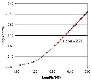Slope of the linear portion of this plot is taken as the overall system gamma (red line in Figure 19). If you would rather skip the math part, here is the spreadsheet that calculates gamma for you in this simple situation. Alternatively, to have log-gamma calculated for you, upload measured values through the GammaCalc page.

Unfortunately, as mentioned above, the OETF characteristics of LCDs are such that a single analytic equation cannot be used to accurately describe their general behavior. Consequently, equations such as eqs. (II-V) may poorly describe the OETF. However, since all computer-controlled systems include video look-up table, three one-dimensional (1D) look-up tables (one for each channel) can be obtained to define the OETF (see Display Color Management). When the GOG functions are replaced with simple one-dimensional LUTs to characterize the display's electro-optical transfer functions, the characterization performance is excellent.

L-star curve:

Some profiling software packages feature several settings for the TRC curve:

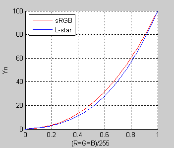
There is not much one can find on the L* curve and it seems that some vendors use proprietary algorithms for the L-star calibration curve and display icc profiles. To get at least a qualitative picture of how the L-star calibration curve looks like, Figure 20 shows the TRCs for both the sRGB and L-star curves in the form of Y(normalized) vs. R'G'B'(normalized) plot - in this section denoted as RGB.

Figure 20: sRGB and L-star TRCs (Yn vs. RGBn)

Relative luminance data (Y) were obtained from the icclu utility of Argyll CMS for both the sRGB and L-star icc profiles. This utility uses the corresponding icc/icm profiles to output XYZ tristimulus or L*a*b* values for batches of input RGB device values. ColorThink Pro can also do the job, although the output data is rounded to only two decimal places.

Note: It should be stressed at this point that sRGB and L-star icc profiles are just color space profiles, theoretical constructs that have nothing to do with display profiles created during calibration/profiling process. As such, these color space profiles could be considered as ideal examples to demonstrate the characteristics of display gamma and L-star profiles.

Visual inspection of Fig. 20 suggests that L-star curve brings more contrast (steepness, higher gamma) into the midtones and highlights (RGB 0.5-0.9). We will also see later that value of gamma is not constant and that it varies along the whole tonal range. Curve characteristics in shadows (< 0.25) are not that clear and additional analysis has to be performed. Overall, both TRC curves are quite similar with no distinct features.

An alternative way to arrive to the similar picture is to calculate luminance values (Y) for the L-star curve from the corresponding values of the CIELAB L-channel (0-100). However, it should be mentioned that typical L-star curve is not identical to the CIELAB L-channel.

Here is the formula for L* to Y transformation: Y = 100 . [(L*+16)/116]3 for Y/100 > 0.008856, Y ∈ <0-100> and Y = 100 . L*/903.3 for Y/100 < 0.008856 Another characteristic plot is shown in Figure 21. Relationship between calculated CIELAB L*-values and the RGB values for a 5-step gray ramp is plotted as L* vs. normalized input RGB. Same ideal sRGB and L-star icc profiles were used, only this time the icclu utility was configured to output L*a*b* values. As one can see, the L-star response is clearly linear in all brightness ranges (blue line). This means that doubling the value of RGB always changes value of L by the factor of two or that by stepping the RGB values by e.g., 10 points will change the L values by a constant increment (in this case by 100/255*10 = 3.9). Also, since incremental changes in L are perceptually uniform, changes from dark to

Figure 21: L-star and ideal sRGB plots

L-star: LAB Lightness vs. RGB inputs for L-star and ideal sRGB gamma gray ramp

bright values in a synthetic grayscale (RGB form 0-255) will be perceived as smooth and uniform. On the other hand, the sRGB curve (or any other typical calibration gamma curve) results in brighter midtones (red curve). Changes of the same 10 RGB points will be perceptually different in shadows, midtones and highlights. For typical calibration gamma curves (2.2, 1.8, sRGB), the shape of the curve in shadows (orange rectangle) will vary depending on monitor black level and on how the calibration algorithm treats the curve in dark areas. Both the linear and typical gamma curves will usually have non-zero luminance at the black while only typical gamma curves may have a higher contrast in that region. Clear distinguishing feature is a convex character of the typical gamma curve in region from about R'G'B'=80 to R'G'B'=200. Real experimental L-star curves are nearly linear.

Before we continue with more detailed analysis, some assumptions have to be made. As we have discussed earlier, LCD display has no underlying physics to follow the power law dependence of luminance vs. digital input. However, we also pointed to the fact that manufacturers build corrections into the display circuitry of the LCD panel to approximate the power function dependence. Such corrections may justify use of the gamma concept. Thus, if the power law dependence is adopted, logarithm of Yn vs. RGBn will be a linear function. Indeed, we often see very good linearity at higher luminance values (~ RGB > 160) as shown earlier in Fig. 19. Unfortunately, for midtones and shadows, this linear relationship (i.e. constant gamma) breaks down. To ensure high accuracy, examples in this section are based on calibrations of higher end Eizo CG19 display using ColorNavigator. Calibration software adjusts only the monitor 10-bit LUT without adding any corrections to the 8-bit video card LUT.

Let's evaluate four different approaches to characterization of TRC curves.

Method 1:

Two types of data were analyzed - experimentally obtained data for both the L-star and the gamma 2.2. calibrated monitor (Tables 3, 5) and ideal color space profile data for both types of curves (Tables 2, 4). For both the sRGB and L-star profiles, relative luminance data (Y) were obtained from the icclu utility of Argyll CMS . It is the same data and curves as in Fig. 20. More specifically, a grayscale RGB ramp (in increments of 5) was used as the input, run through the icc profile to get the corresponding XYZ tristimulus data. Y-component of the tristimulus output and the input RGB data were used in the curve fitting examples. The digital input range (0-255) was divided into smaller subranges as shown in Tables 2 to 5 (column 1). Data points in each subrange were fitted to a general power function and the power coefficient γ was recorded in column 2. Root mean squared error (the square root of the mean square error or

the standard error) is shown in column 3. Linear regression was performed on the log-log scale for the same data points and slope of the fitted line (γ) is listed in column 4. This would correspond to the so called log-log gamma. The corresponding RMSE data are shown in column 5. Gamma values calculated in columns 2 and 4 will obviously be different. It should not matter which definition of gamma we choose as long as we stay consistent. Remember, the log-log(γ) is the definition used in display calibration where linear regression is done in the logarithmic domain.

Following are some observations made from Tables 2-5:

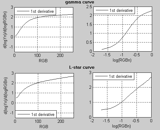
Method 2:

To further assess differences between the two calibration curves, relative luminance values (Y ∈ <0-100>) were either measured or calculated using the icclu CMS utility. Polynomial fit was done on the data (linear and log-log scale) followed by the plot and data analysis. In general, the first derivative of the fitted function (logYn vs. RGB or logYn vs. logRGBn ) reflects well the type of the TRC curve. Plots of d(logYn)/d(logRGBn) vs. RGB and d(logYn)/d(logRGBn) vs. logRGBn are shown in Fig. 22. L-star curve has extensive linear parts in the logRGBn plot and continuously decreasing "gamma" in the RGB plot. On the other hand, the plot of "classical" gamma curve has a typical S-shape in the logRGBn plot while the RGB plot shows more constant gamma in highlights. However, as indicated earlier, more data is needed to formulate any general characteristics from these plots. Due to the larger size of the images, the corresponding analysis is available in this document (v. 1.0) (check here for the latest version).

Figure 22: 1st derivatives of logYn vs. RGB or logRGBn for L-star and gamma TRCs

Method 3:

This method provides only a qualitative comparison between two or more TRC curves. All are subtracted from a reference TRC (in our case the ideal camera sRGB TRC curve). When display TRC curve is also sRGB, a straight line from 0 to 1 will

Figure 23: L-curves subtracted from camera sRGB γ
(place mouse over the image to toggle)

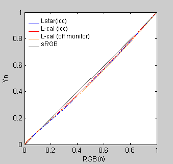result from the subtraction. This is the case shown in Fig. 23 (black diagonal line). Other three lines are TRCs of the L-star curves relative to sRGB curve. Blue line shows an L-star curve coming from the L-star icc profile, the red line is an L-star curve coming from the icc profile of calibrated/profiled monitor, and the orange line is the experimentally measured TRC based on the same icc profile. Measurement was done directly off the screen using 5-step gray ramp. In general, the L-star curves make midtones slightly darker than the typical gamma based TRCs. We have already seen the same trend in Fig. 21. For more detailed inspection of these curves, place mouse over the image in Fig. 23. On the toggled image, differences from the sRGB TRC are exaggerated four times. As one can see, the major differences from "classical" gamma curves are in midtones, specifically in R'G'B' ranges of 25-100 (8-bit encoding). It is mostly the curve steepness (contrast) that differentiates the curves from each other.

Method 4:

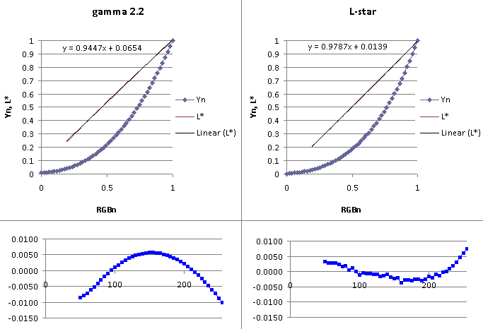
The relationship between measured tristimulus Y-values (normalized) and RGB normalized values for a 5-step gray ramp is plotted in Fig. 24 as Yn vs. RGBn. Left panel shows data obtained from L-star calibrated Eizo CG19 monitor, the right panel shows data obtained from similar gamma 2.2 calibration both using ColorNavigator and the X-rite DTP-94 colorimeter. In both cases, the Y-values were also transformed into L* values of the CIELAB color space.

Here is the formula for Y to L* transformation: L* = 116 . (Y/100)1/3 - 16 for Y/100 > 0.008856, Y ∈ <0-100> and L* = 903.3 . Y/100 for Y/100 < 0.008856 Least squares fitting method was used to fit a line to the L* vs. RGBn function. Fitted straight line shown in the right panel (in black) is nearly identical to the original L* vs. RGBn function. On the other hand, the linear regression performed on the "classical' gamma curve (left panel) shows hints of deviation from the straight line. The corresponding sums of squares due to error (SSEs) are 0.0003 (L-star) and 0.0010 (gamma 2.2.). Analysis of residuals reveals further details of the fit. While residuals for the L-star curve have generally monotonic concave character, residuals of the gamma curve have a characteristic convex shape typical for other measured or theoretical gamma curves. Due to the uncertainty of curve behavior in the dark areas, evaluate only parts of the plot starting from about R'G'B'=50 (RGBn=0.2) and up. Here is the Excel worksheet that performs all the calculations.

Figure 24: Linear fit to L* vs. RGB for gamma and L-star TRCs with plotted residuals

(top)↑Links and References:

Last update : April 15, 2009